Introduction and Motivation

The goal of this blog post is to give a detailed summary of the Metropolis-Hastings algorithm, which is a method for sampling data points from a probability distribution. It is mainly used when applying Monte Carlo methods. The principle behind these methods is to use random sampling when trying to solve deterministic problems. For example, to approximate the number \pi we can generate uniform samples from the unit square and multiply by four the proportion of points inside the quadrant, i.e. having a distance lower than 1 from the origin. By the law of large numbers this approximation will converge to \pi. 

One main application of the Monte Carlo method is when facing the objective of computing the integral I(f)=\int_{x}f(x)p(x)dx,where p(x) is a probability density function. In the case, where I(f) is intractable, we can approach this task by sampling x_1,\ldots ,x_n\sim p(x) and using I_{N}(f)=\sum_{i=1}^{N}f(x_i)as an estimator for I(f). I_N(f) is known to be consistent, unbiased, and asymptotically normal, which are all indeed very nice properties for an estimator.

A main field in statistics where we face such a problem is with Bayesian Inference. Suppose that we want to estimate an unknown parameter x\in \mathcal{X} based on data y\in \mathcal{Y}. An example for a Bayes estimator is the expected value of the posterior distribution, i.e. \int_{x}xp(x\mid y)dx. It is often the case where this integral is intractable, and therefore using Monte Carlo will come in handy.

But what if we can’t sample from the posterior distribution? Or perhaps the distribution is known only up to a normalizing constant. In this case we can use the Metropolis-Hastings algorithm to produce a sample. It belongs to a class of algorithms called Markov chain Monte Carlo (MCMC), which is based on using Markov chains to generate samples from any probability distribution, even when its density is known only up to a normalizing constant. 

In the rest of the post, I will present the Metropolis-Hastings algorithm and give proof as to why it works. In order to do so, I will introduce the subject of Markov chains, and dive into its concepts which are necessary for understanding the idea behind MCMC.

The Algorithm

When I first saw the algorithm, I was amazed by its simplicity. It took just several lines of code to implement, and when I tried it for the first time, it worked like a charm.

Let p(x) be the distribution that we wish to sample from. We’ll call it the target distribution. Notice that we don’t know how to directly generate samples from p(x), and furthermore we know it up to a normalizing constant. In each iteration, we sample a candidate from a proposal distribution {q(x^*\mid x),} which is a distribution that we can easily sample from. q(x^*\mid x) should share the same support as p(x), i.e. the two distributions should have the same range of x-values. The Metropolis-Hastings algorithm is defined as

1. Initialize x_0
2. For i=0 to N-1
   • Sample u\sim \mathcal{U}(0,1).
   • Sample x^*\sim q(x^*\mid x_i).
   • If u\leq \mathcal{A}(x_i ,x^*)=\min \{1,\frac{p(x^*)q(x_i\mid x^*)}{p(x_i)q(x^*\mid x_i)}\} \newline           x_{i+1}=x^* \newlineelse \newline           x_{i+1}=x_i

There are a few important details to notice here, which I will elaborate on later in this post. First, the proposal distribution is conditioned on the latest sample x_i. Second, given a realization of x^*, we accept it with probability \mathcal{A}(x_i,x^*), which we define as the acceptance probability, otherwise we stay in x_i. If we take a symmetric distribution to be our proposal distribution, then the two terms related to it in the acceptance probability cancel out, and we’re left with the ratio of the target distribution at the points x^* and x_i, meaning that \mathcal{A}(x_i,x^*) becomes \min \{1,\frac{p(x^*)}{p(x_i)}\}.

We will use the following examples of p(x) and q(x^*\mid x) throughout the post.

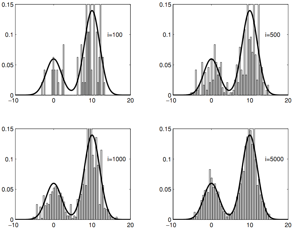
• p(x)\propto 0.3e^{-0.2x^{2}}+0.7e^{-0.2(x-10)^2}
• q(x^{*}\mid x_i)\sim \mathcal{N}(x_i ,\sigma^{2})

Figure 2 shows that with more iterations, the empirical distribution will appear closer to the target distribution. In fact, it is guaranteed that the sample distribution of x_0,\ldots ,x_N converges to p(x). At a first glance, it is very surprising that this is true, and not at all intuitive (at least for me it wasn’t). Proving it relies on the theory of Markov Chains, so to be able to do so, I will first introduce the subject.

Markov Chains

A Markov chain is a stochastic process which is characterized by the property that each transition in the process is dependent solely on the current state, and not on its past. This is called the Markov property. For simplicity, let’s assume that our process has discrete time steps and a finite state space, i.e. x_i \isin \{1,\ldots ,s\}. Thus, by the Markov property we have that P(X_{t+1} \mid X_t,X_{t-1},\ldots ,X_0)=P(X_{t+1}\mid X_t)  ,  \forall t\geq 0.In this section we’ll learn about the conditions in which a Markov Chain, after enough time steps, will produce a sample with an empirical distribution sufficiently close to a particular probability distribution. Later on we’ll see that the Metropolis-Hastings algorithm generates a Markov chain that follows these conditions, and we’ll prove that indeed it converges to our target distribution.

We’ll discuss Markov Chains that are time homogenous, meaning that the probability of moving from one state to another is time invariant, i.e. P(X_{t+1}\mid X_t)=P(X_1\mid X_0)  ,  \forall t\geq 0.I will go over some basic concepts in Markov chains through some examples. Let’s start with an example of a three-states Markov chain (s=3) which is depicted in the following transition graph.

Once the process is in a given state, the arches coming out of it represent the probability of moving to another state in the next time step. The same information, which basically describes the Markov chain, can be represented in a transition matrix T, where its (i,j) element is the probability of moving from state i to state j, i.e. T_{ij}=P(X_{t+1}=j\mid X_t=i). Hence in our example T=\begin{pmatrix}0 &  1 & 0 \\ 0 & 0.1 & 0.9 \\ 0.6 & 0.4 & 0 \end{pmatrix}.

Limit Distribution

An interesting question about Markov chains is how will it behave after many time steps. In particular, what is the probability to be in state j\in \{1,\ldots ,s\}  after infinite steps? First let’s define {\pi_t(j)=P(X_t=j)} , which is the probability of being in state j at time step t. What will then be \pi_1? Obviously, it depends on the initial state of the process. So we’ll assume that the initial state is randomized using a known probability vector \pi_0. Therefore we can use the law of total probability to calculate each element in \pi_1 by P(X_1=j)=\sum_{i=1}^{3}P(X_1=j\mid X_0=i)\pi_0(i). Alternatively, we can use a vector form, \pi_1=\pi_0T. We can proceed with this calculation iteratively to get \pi_2=\pi_1T=\pi_0TT. For any arbitrary time t we have, \pi_t=\pi_0\underbrace{T\cdots T}_{t  \text{times}}=\pi_0T^{(t)}. Now we can formally define the Limit distribution of a Markov chain as \pi_\infty =\lim\limits_{t\rarr \infty}\pi_t=\lim\limits_{t\rarr \infty}\pi_0T^{(t)}.There are a few fundamental questions about Markov chains, including: Does a limit distribution exist? Or is it unique?

In our example the limit distribution does mysteriously exist and is equal to \pi_\infty=(0.2,0.4,0.4). Furthermore, it is unique, regardless of \pi_0! Meaning that it doesn’t matter where we start the stochastic process, if we stop the system at the abstract time of infinity, it will be in state 1, 2, or 3 with probabilities 0.2, 0.4, and 0.4, respectively. For the rest of this section, we will discuss the conditions that a Markov chain magically has a unique limit distribution. To do so, I will introduce some key definitions through a couple of (contrary) examples.

Irreduciblity

Consider the following Markov chain with six states.

It is actually as if we duplicated the Markov chain in the previous example and made no feasible transitions between the two. It is easy to see that the limit distribution here depends on the initial state of the process, therefore it is not unique. If we start in states 1, 2, or 3, we will never reach states 4, 5, nor 6, and the limit distribution will be (0.2,0.4,0.4,0,0,0). On the other hand, if we start in states 4, 5, or 6, we will never reach states 1, 2, nor 3, and the limit distribution will be (0,0,0,0.2,0.4,0.4). We can learn that the Markov chain in the former example possessed an important characteristic, essential for having a unique limit distribution, which is described in the following definition.

Definition 1: In an irreducible Markov chain, each state is reachable from any other state, in a finite number of steps.

The chain in the current example is clearly not irreducible.

Periodicity

To introduce the next concept, consider the following Markov chain with four states.

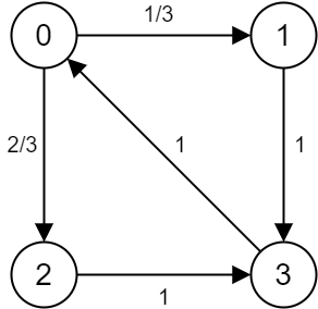
Suppose we start the stochastic process in state 0, i.e \pi_0=(1,0,0,0). From the transition graph we understand that \pi_1=(0,\frac{1}{3},\frac{2}{3},0), and at t=2 we will surely arrive at state 3, followed by state 0 at t=3, meaning that \pi_2=(0,0,0, 1) and \pi_3=(1,0,0,0). Notice that we are back to the initial state, hence for the following time steps, we repeatedly get \pi_4=(0,\frac{1}{3},\frac{2}{3},0), \pi_5=(0,0,0,1) and \pi_6=(1,0,0,0), and so on. In other words, after 3 steps we will always go back to state 0. We can easily see that the process will surely go back to the same state after a multiplier of 3 steps. Clearly this Markov chain does not converge to any limit distribution. This brings me to the following definitions.

Definition 2: A state i has a period \bm{k} if any return to state i must occur in k time steps. Formally, the period of state i is defined as k=\gcd \{n:P(X_n=i\mid X_0=i)>0\}.Definition 3: A Markov chain is aperiodic if the period of all its states is 1.

An observation that will be useful later is that in an irreducible Markov chain all the states have the same period. We will soon see how irreduciblity and aperiodicity play an important role in a fundamental theorem regarding the limit distribution of Markov chains. 

Stationary

The last definition before we continue to this theorem is:

Definition 4: \pi is the stationary distribution of a Markov chain with Transition matrix T if \pi=\pi T, and \pi is a probability vector.

We can look at it as if T maintains \pi. In other words, if we randomize our initial state using the vector \pi, or if miraculously a transition probability for some time step n is equal to \pi, then for any t>n we have \pi_t=\pi. In that case we say that the Markov chain reached its steady state, or equilibrium. From the perspective of a single state, under a stationary distribution \pi, we have for each state i, \pi(i)=\sum_{j}\pi(j)T_{ji},also known as the global balanced equations. Subtracting \pi(i)T_{ii} will give us, \pi(i)(1-T_{ii})=\sum_{j\neq i}\pi(j)T_{ji}, which can be interpreted as the flux out of state i equals the flux into state i.

In our first example, in addition to being the limit distribution, (0.2,0.4,0.4) is also stationary. As we’ll see immediately, it is not by sheer coincidence.

Basic Limit Theorem

A fundamental theorem in Markov chain theory is the Basic Limit Theorem, which unites all of the concepts we’ve learned so far.

Theorem 1: If a Markov chain is irreducible and aperiodic, then:

1. \exist !\pi=(\pi_1,\ldots ,\pi_s) stationary distribution
2. \lim\limits_{t\rarr \infty}P(X_t=i)=\pi_i  ,  \forall i

That is, the chain will converge to the unique stationary distribution.

Something to keep in mind is that our goal is to generate a sample from a target distribution p(x), so the main take-away from this theorem is: to achieve this goal we can construct an irreducible and aperiodic Markov chain with a stationary distribution equal to p(x).

Theorem 1 guarantees that this process will converge to the desired distribution. But how can we make sure that the target distribution is indeed stationary with regards to this Markov chain? This brings me to the next concept.

Reversibility

Definition 5: A Markov chain is said to be reversible if there is a probability distribution \pi over its states such that  \pi (i)T_{ij}=\pi (j)T_{ji}  ,  \forall (i,j).Also known as  reversibility / detailed balance condition.

Theorem 2: A sufficient, but not necessary condition for \pi to be a stationary distribution of a Markov chain with transition matrix T is the detailed balance condition.

It is easy to see that the detailed balanced equations are a sufficient condition for the global balanced equations, as it requires for each pair of states (i,j), that the flux from i to j equals to the flux from j to i. This differs from the global balanced equations, which ensures that the flux in and out of any state i is the same.

This helps us greatly since if we can construct an irreducible, aperiodic, and reversible Markov chain with regards to a target distribution p(x), then according to theorems 1 and 2, the chain will converge to this distribution. As we will see shortly, this is the essence of the Markov chain Monte Carlo methods, and particularly the Metropolis-Hastings algorithm.

Back to the Algorithm

Before diving back into the algorithm, I will address the fact that the above theorems also apply to the case where the state space is continuous, we just need to make the proper modifications for it. In particular, to reflect the transition distribution from state to state we will use a Transition Kernel K(X_{t+1}\mid X_t), instead of a Transition matrix T. Moreover, to describe the distribution over the state space at time t, we will replace the vector probability \pi_t with a density function.

Clearly, the stochastic process generated from the Metropolis-Hastings algorithm is a Markov chain. The Markov property is derived by the fact that the distribution of the next state depends solely on the current state, and not on its past. Obviously the chain is irreducible since at each step we have a positive probability to reach any range in the support of the proposal distribution, which essentially defines the state space of the chain. In addition, for some state x', we will get an acceptance probability smaller than one, hence the chain will stay at x' with a positive probability, and therefore its period is 1. As mentioned earlier, in an irreducible Markov chain all the states have the same period. Therefore in this Markov chain, all of the states have a period of 1, meaning that it is aperiodic.

Thus we have an irreducible and aperiodic Markov chain, and therefore by the basic limit theorem it will converge to a unique stationary distribution. Clearly the algorithm developers constructed it in such a way that the stationary distribution equals the target distribution. If we show that this is truly the case then we would prove that the algorithm works. Using what we have learned on reversible Markov chains, we can show that the Markov chain is reversible with regards to p(x), and according to theorem 2, it will show that p(x) is the stationary distribution. Put differently, we will prove that the transition kernel of the Markov chain holds the detailed balance condition with regards to the target distribution p(x), that is p(x_i)K(x_{i+1}\mid x_i)=p(x_{i+1})K(x_i\mid x_{i+1}),  \forall (x_i,x_{i+1}).

Transition Kernel

We can express the transition kernel as K(x_{i+1}\mid x_i)=q(x_{i+1}\mid x_i)\mathcal{A}(x_i,x_{i+1})+\delta_{x_i}(x_{i+1})r(x_i).Where r(x_i)=P(\text{reject}  x^*)=1-\int \mathcal{A}(x_i,s)q(s\mid x_i)ds is the probability of rejecting x^* that is sampled from the proposal distribution, and \delta_{x_i} denotes the delta-Dirac mass located at x_i. Delta-Dirac is a generalized function which can be used in describing random variables with a mixture of a continuous part and a discrete part. In particular, it is characterized by returning the value of 0 anywhere besides its mass, and being integrated to 1, which allows us to write a valid density function that integrates to 1. In our case, the discrete part is at x_i since there is a positive probability to stay in the same state, namely r(x_i). For x_{i+1}\neq x_i, \delta_{x_i}(x_{i+1}) zeros out and we stay with the proposal density at x_{i+1} multiplied by the probability to accept it.

Going back to our example.

• p(x)\propto 0.3e^{-0.2x^2}+0.7e^{-0.2(x-10)^2}
• q(x^*\mid x_i)\sim \mathcal{N}(x_i,\sigma^2)

This is a schematic representation of the transition kernel where x_i=7 and \sigma ^2=10.

We see the Gaussian curve around x_i, yet the transition kernel “punishes” those parts of the support where the density of the target distribution is smaller than p(x_i). If we sum up the area between the green and red line, we will get the probability of rejecting x^* and remaining in x_i, which is reflected in the mass point at x_i. In the other parts, where the acceptance probability is 1, the transition kernel is bounded by the proposal density.

Last Step in the Proof

Now that we fully expressed and understood the transition kernel of the Markov chain generated by the Metropolis-Hastings algorithm, the final step in proving why it works is quite simple. We just need to show that the detailed balance equation is true. For the case where x_i=x_{i+1} it is trivial. For x_i\neq x_{i+1} we have, p(x_i)K(x_{i+1}\mid x_i)=p(x_i)q(x_{i+1}\mid x_i)\mathcal{A}(x_i,x_{i+1})=\newline \min\{1,\frac{p(x_{i+1})q( \,x_i\mid x_{i+1})}{p(x_i)q(x_{i+1}\mid x_i)}\}p(x_i)q(x_{i+1}\mid x_i)=\newline \min\{p(x_i)q(x_{i+1}\mid x_i),p(x_{i+1})q( \,x_i\mid x_{i+1})\}.If we were to do the same for p(x_{i+1})K(x_i\mid x_{i+1}) we would receive the same expression, thus the proof is concluded.

Final remarks

There are a few final points worth mentioning regarding the use of Metropolis-Hastings algorithm.

Proposal Distribution

The way we choose the proposal distribution is very important for the convergence of the Markov chain, as illustrated in the following figure.

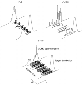
If we set the proposal distribution too centered around x_i, then it will take us a long time to explore the state space since we will get “stuck” around high density areas. As shown in figure 7, this is what happens if the variance of the Gaussian proposal distribution is 1, which is too small. On the other hand, when setting it too high, for example at 100, if the chain is in a high density area, we would frequently reject new samples. Alternatively, if the chain is in a low density area, we would immediately be thrown away from there without exploring it enough. The trick is to find the “sweet spot”, that is the optimal parameters to allow you exploring the state space in an efficient manner, as illustrated when choosing the variance to be 10.

Auto-Correlation and Convergence

Another thing to consider is that the samples generated from the algorithm are auto-correlated, as expected from a Markov chain. Obviously the correlation decreases as the time difference between the samples increases. This should not be of concern when taking the entire sample as a whole, after enough iterations have been conducted and the Markov chain has reached its steady state. Until that point of equilibrium, the chain is in a Burn in phase and we should be careful not to stop the process at that time.

Summary

To summarize, we learned that the Metropolis-Hastings belongs to a class of algorithms called Markov chain Monte Carlo. These algorithms are used to generate a sample of a random variable by producing a special type of Markov chain, in particular, an irreducible and aperiodic. With the help of Markov chains theory, we’ve proven that the Metropolis-Hastings converges to the target distribution by showing that it equals the stationary distribution of the process produced by the algorithm. In addition, we discussed some important points to consider when applying the algorithm.

Lastly, I would like to thank Christophe Andrieu et al. for their insightful introduction paper to MCMC for Machine Learning.

 

---

 

About the author:

Dan Bendel is a Data Scientist in the Data Analysis & Algorithms group at SimilarWeb.