Calculating Damerau-Levenshtein distance using trie structure in a distributed environment
Introduction
Analysis of textual data can be a highly time consuming process, especially regarding datasets of great volume. Thus, any improvement to the speed of existing text analysis algorithms can be significant. In some cases, accelerating the runtime can turn an analysis from incomputable to feasible within the constraints of a given data cluster.
A staple algorithm of text comparison is the Damerau-Levenshtein measurement of edit distance (DL metric) between two strings of text [reference]. In this blog post, we will be using this algorithm to match a small set of words against a very large set of words. We will compare the efficiency of calculating the DL metric using a naive approach vs using the trie data structure, as presented in the blog post by Steve Hanov [reference]. We will also show an efficient way to distribute the DL metric calculation for additional improvement. This blog post will present the necessary code for the analysis, to facilitate understanding and for reuse in your own projects.
What will be covered in this post:
- Results for the baseline straightforward edit distance, both locally and distributed
- Results for the trie based edit distance, both locally and distributed
- Possible improvements and scaling data results
Setup
Note: The presented code relies on the spark distributed infrastructure, and is written in pyspark.
Let’s load a freely available data set of 1M words from the FastText website:
After we perform the lowercase transformation, the remaining data consists of 831,375 words (still pretty large for toying around).
Baseline edit distance
Now, let’s define the well known Damerau-Levenshtein function:
And test to see if it works:
Great! Working as expected (the edit distance is 2, due to the ‘ar’ and ‘eb’ transpositions).
Now, let’s define a small set of words we would like to run against the whole data set. The idea here is not to calculate the whole set of distances (|small_set| x |large_set|), but rather filter those results according to a given maximum distance:
In this small example, we have defined 10 words and a maximum edit distance of 1.
All right! Let’s incorporate all of the previous code and run the DL metric measurement against the large set (~830K set of words):
On our local server, the total runtime was 6 minutes 22 seconds, as the code uses a for loop to iterate through all the words. So, this runtime is the baseline benchmark to beat.
If you look at this naive code, you will notice an obvious potential improvement. We should check whether the difference between word lengths is small enough to be worth calculating the DL metric in the first place. In other words, for a given maximum distance, the difference between word lengths should not exceed that maximum distance:
A good start! Almost 3 times faster with just this small addition of code!
Distributing the DL metric calculation
Now let’s move from running the code locally to utilizing our distributed environment. The new code creates a spark RDD object from the data set and broadcasts all relevant variables to the workers:
Note: We chose to divide our data into 30 partitions for this post, but it depends on your cluster.
Here we define our mapper function to calculate DL metric measurement separately on each partition:
And here we run our distributed code:
We can validate that the results are identical with the local run result, which is the case here.
Let’s examine the statistics of the distributed calculation runtimes:

As you can see, the median runtime is ~6 seconds. This runtime is a bit slower than the expected linear advantage of 30 simultaneous runs (as our local run took ~134 seconds). This overhead is not the time it takes to perform the reduce operation nor is it the time required for sending and receiving the data to and from the local machine. So, we attribute it to the difference in compute power between the driver and workers of our clusters, your results may vary.
Utilizing the trie data structure
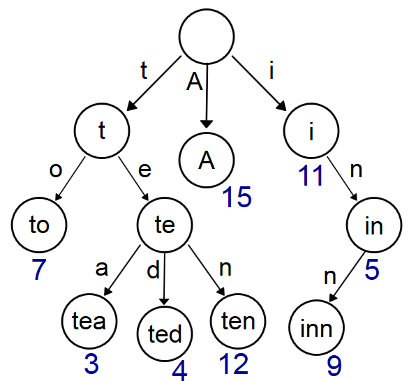
But what if we want even faster runs? For a very large dataset of tens of millions of strings, this calculation is obviously not going to be completed within 6 seconds. The improvement we want is to introduce a trie into the calculation. A trie [reference] is a prefix tree of strings, wherein strings that share the same prefix are contained within the same branch. Utilizing the trie structure allows calculating the distance of those strings while simultaneously enforcing the maximum distance limit.
There are a few caveats to using a trie which you should pay attention to before attempting implementation:
- A trie must be built before it can be used. In this solution, the trie is built everytime before running the search process.
- If there are many unique characters in the strings (Chinese characters for example), a trie is going to take a long time to build and will require a considerable amount of memory, which will generally slow things down.
- The trie search process is recursive and thus computation time will grow exponentially with the maximum distance limit.
The decision to use the trie structure was inspired by the solution presented in Steve’s post [reference], so we have implemented the trie code almost exactly the same, except for two important changes:
- We extended the solution to allow for Damerau-Levenshtein distance calculation instead of plain Levenshtein (The Damerau-Levenshtein also allows character transpositions).
- We decided to use an available trie python package called datrie.
Note: More details about the trie structure generation algorithm are available in Steve’s post [reference]
Let’s create a class which will handle the trie based distance search:
Note: The DamerauLevenshteinTrie class supports the max_calc_flag boolean as initialization parameter. This flag takes string lengths into account when considering continuing to a lower trie branch.
Now we can repeat the previous process, while replacing the exhaustive “for loops” with the trie recursive search process. Starting with the local run:
4 minutes and 14 seconds! (The results are in unicode due to datrie input requirements). The new runtime is less than 6 minutes, but it’s not really the improvement we were hoping for. Why is this so slow? Since we have built the local trie already, we can reuse it for the distance search:
Wow, less than a second! As you can see, all of the time was spent on building the local trie.
Encouraged by this result, we return to the distributed execution, creating smaller tries for each partition and then reducing the results back. Here, we define another mapping function:
OK, let’s test the running time:

The results are identical to the local run again, which is good. Let’s see statistics of partitioned tasks:
A median of ~1 second, much faster than the local run of 234 seconds! So, building 30 smaller tries actually introduced a non linear running time reduction. Compared to the straightforward run, there’s a ~6 times improvement. Actually, increasing the number of partitions will create even smaller tries and will further reduce the runtime. Obviously, reducing runtime to lower than a second is not really interesting, but this new implementation can support a much larger target set and still return results within a reasonable time.
Additional tweaks
A few further optimizations to consider:
- The max_calc_flag boolean flag that takes string lengths into account did not introduce significant improvement.
- It is possible to repartition the data in a smart way that will create narrow tries, possibly reducing running time while searching.
- The datrie package is fast in general, but the search could be even faster if there was a way to return edges given a prefix straight from the package (in C) instead of using a python list comprehension (wasn’t tested in the scope of this blog post).
- We have also witnessed the enormous advantage of searching a pre-built trie, therefore it is possible to build small tries and save them to a centralized storage for later reuse
Regarding the second bullet, here’s an example of one way of reorganizing the data for quicker trie builds. Here, we take the prefix of up to the first 3 letters to be the keys for organizing our data:

A median of ~0.5 seconds. By regrouping the data we succeeded to reduce running times even more.
One final tweak would be to store small tries on a shared storage (S3 for example) for later use. This can potentially save even more runtime being dependent on loading the trie from file only. With datrie we can dump a pickle of the trie, with other tries you will need to make sure they are pickle-able.
Let’s define two new functions:
We want every partition to be saved by the worker:
Since we have set up 30 partitions, to get the partition number for each key we will hash it and return modulo 30. This way, we group by key and build tries for that partition.
Now we want to use these saved tries:

There you go, works well and fast! Remember, the datrie package is fast, but it lacks some features which could reduce the amount of python loops in the process.
Conclusion
The baseline runtime for calculating the DL metric (6:22 minutes) is quite long for the given task and size of the target dataset (~830K words), so there is definitely cause not to use the naive approach and to apply optimization. This parallelizable task really lends itself to be partitioned so using a distributed calculation is an obvious improvement to implement. However, the major reduction in runtime is associated with transforming our data into the trie structure (the process sped up by ~12 fold). All in all, by combining all the aforementioned improvements to the baseline calculation, we transformed this rather cumbersome algorithm into a more streamlined process that is able to support a dataset larger by several order of magnitude. We hope you will find these code snippets useful in your respective research.
About the author:
Philip Khripkov is a Data Scientist in the Data Analysis & Algorithms group at SimilarWeb.